Back • Return Home
It's Vortices! Vortices All The Way Down!
This document is a continuation of the previous article, The Universe: A Play In Four Acts. Here we will try to extend the patterns already given into "higher dimensions" and show their general application to "physics". This may sound complicated, but we will try to make it as simple as possible to understand. Only basic Arithmetic (i.e.: the ability to add, subtract, divide, and multiply) and basic Geometry (i.e.: the ability to recognize shapes) will be needed. It may seem like a lot of text, but please have patience for it and try to visualize what is described as you read. You might want to keep some basic tools handy (i.e.: a pencil, some paper, a ruler / straight edge, a drafting compass, and a calculator)! There are also quite a few images, so if your internet collection is slow, it may take a moment to load. If an image returns a broken link, right-click it and select "Reload Image".
Contents
• Part 1: The Basics of Graphing
• Part 2: The Basics of Tessellations
• Part 3: The Basics of Topological Vector Spaces
• Part 4: The Unified Field
Part 1: The Basics of Graphing
There is a balance or mirroring amongst many different aspects of mathematics, including within the operations of arithmetic. We can use one operation to check the validity of an equation by changing it into another with a complementary operation. For example:
2 + 1 = 3 and 3 - 2 = 1 or 3 - 1 = 2
Notice that addition and subtraction describe scenarios which are inverted from one another (e.g.: combining and separating). Each "undoes" the other. Therefore, we refer to them as "inverse operations".
Similarly, multiplication and division are also inverse operations. For example:
2 × 3 = 6 and 6 ÷ 2 = 3 or 6 ÷ 3 = 2
Again, each "undoes" the other.
In the case of addition and multiplication, changing the order of the numbers does not change the final result. We would say that they are "commutative". For example:
2 + 3 = 3 + 2
2 × 3 = 3 × 2
Subtraction and division do not usually share this property. We would say that they are "non-commutative". For example:
6 - 3 ≠ 3 - 6
6 ÷ 2 ≠ 2 ÷ 6
If we subtract a larger number from a smaller one, then we introduce a new kind of number, a "negative number". For example:
2 - 3 = -1
read as "two minus three equals negative one"
In this case, two is less than three, but there is still a difference of one between them.
It is easy to think of "negative numbers" as symbolizing the idea of debt (i.e.: something owed to another). In this sense, they are "less than zero". As an analogy, if someone has "negative dollars" in their bank account, not only do they not have any money, but they also owe the bank!
Just as there are negative numbers, there are also "positive numbers", which are synonymous with the regular counting numbers. To put it another way, we usually think of numbers like 1, 2, 3, 4, etc. as being the same as +1, +2, +3, +4, etc. The "sign" of a number determines what it is: Negative numbers have a "minus sign" (-) in front of them, while positive numbers can have a "plus sign" (+) in front of them, or nothing at all.
Like addition and subtraction, negative numbers and positive numbers "undo" each other. For example:
-2 + 2 = 0
read as "negative two plus two equals zero"
If we combine a negative two and a positive two, they cancel each other out leaving zero. One might use the analogy of negative two being like a hole in the ground, and the positive two being like a mound of dirt that can fill it completely. Any two numbers which add together to equal zero like this are called "additive inverses".
When taken together as a set, all negative numbers and positive numbers are known as "integers". We can represent all integers on a structure called a "number line". It looks like this:
Negative numbers are to the left of 0 and positive numbers are to the right of 0. Therefore, moving to the right would be like adding, while moving to the left would be like subtracting. The arrows at each end show that the line can be extended as far as is necessary in order to include ever larger numbers. [If we want to be extra-fancy, mathematically we would say that the line has "infinite extension", with the negative numbers going towards "negative infinity" (symbolized by -∞) and the positive numbers going towards "positive infinity" (symbolized by +∞).]
We can represent any number on the number line as a "point" or dot. For example:
Notice the green dot on -2.
Likewise, the number associated with the point is called a "coordinate". The number line is considered a "1-dimensional space" because it only takes one coordinate (or number) to represent any location (or point) on that line. To put it more simply, one coordinate = one dimensional.
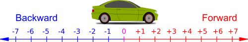
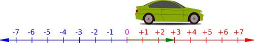
We can use this 1-dimensional space to model many things. For example, if our number line was representative of a driveway, then a positive number could describe the forward motion of a car going into that driveway, while a negative number could describe the backwards motion of a car reversing out of that same driveway:
Any location that the car can take within the driveway can be represented as a single point along a number line. This is because the car is only moving forwards and backwards in this situation. We could say that its motion is "1-dimensional" (i.e.: only forwards or backwards along a line).
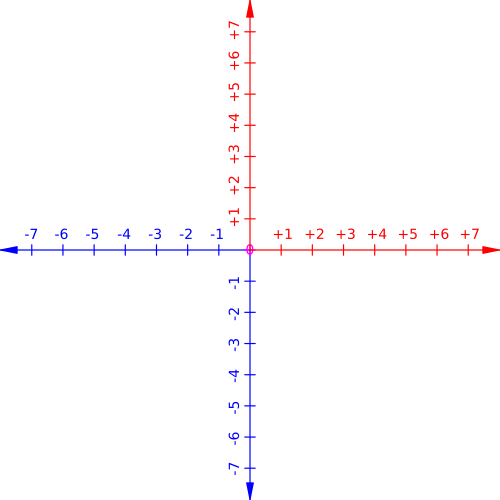
Now, let's take two number lines and overlay them to make a cross. Both number lines will be "perpendicular" to each other (i.e.: 90-degrees away from one another), like this:
This is called a "Cartesian plane" (after the famous French mathematician René Descartes). We will show how this can be an incredibly useful tool for visualizing various kinds of relationships, but first, there are several things to notice about it:
• There is one number line moving horizontally. We will call it the "X-axis".
• There is another number line moving vertically. We will call it the "Y-axis".
• The zeroes of each number line overlap. We will call it the "origin".
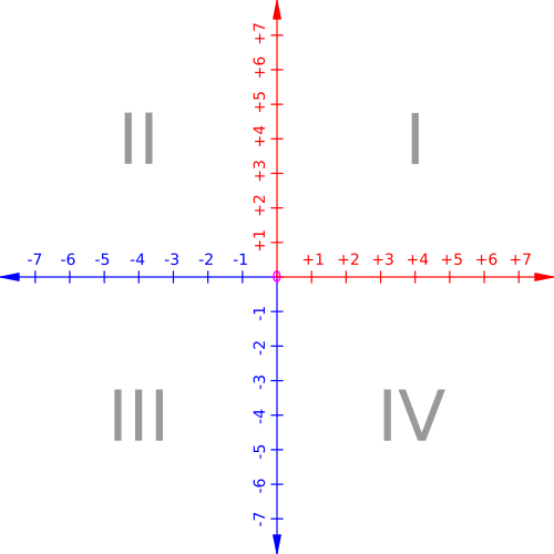
The number lines (or "X and Y axes") make four distinct zones called "quadrants":
Moving counter-clockwise, the quadrants are labeled I, II, III, and IV.
The X and Y axes also imply a grid:
Any point on the grid can be represented by two numbers. These two numbers are called an "ordered pair". For example, they are written like this:
(3, 2)
The first number tells us how far to move left or right along the X-axis. We will call it the "x-coordinate" [or to be extra-fancy, the "abscissa"]. The second number tells us how far to move up or down along the Y-axis. We will call it the "y-coordinate" [or to be extra-fancy, the "ordinate"]. For example:
Here the green dot represents the ordered pair (3, 2). In this case, 3 is the x-coordinate, while 2 is the y-coordinate. It tells us to move 3 units to the right and 2 units up from the origin in order to reach that point. The zero at the center of the grid is called the "origin" because this is always were we begin when interpreting an ordered pair! The quadrant that a point ends up in is determined by the sign of the numbers within the ordered pair (e.g.: since 3 and 2 are both positive, the point that they describe is within quadrant I).
Because it takes two coordinates to locate any point within it, the Cartesian plane is considered a "2-dimensional space". Again, two coordinates = two dimensional. We will come back to the Cartesian plane soon enough, but for now, let's take a look at sequences...
The regular counting numbers make a sequence:
1, 2, 3, 4, 5, 6, 7, 8, etc.
This is called an "arithmetic progression" because we just need to add a number (called the "common difference") in order to get the next number within the sequence. In this case, we are repeatedly adding 1:
1
1 + 1 = 2
2 + 1 = 3
3 + 1 = 4
4 + 1 = 5
5 + 1 = 6
6 + 1 = 7
7 + 1 = 8
...etc.
Therefore, 1 is the "common difference". The reason that it is called a "common difference" is because any number within the sequence minus the number before it will always give the same number. To put it another way, it is the "difference" that is "common" to them all.
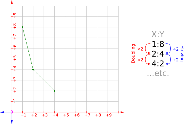
Here is another kind of sequence:
1, 2, 4, 8, 16, 32, 64, 128, etc.
This is called a "geometric progression". We can get the next number within the sequence by continuously multiplying by another number (called the "common ratio"). In this case, we are repeatedly multiplying by 2:
1
1 × 2 = 2
2 × 2 = 4
4 × 2 = 8
8 × 2 = 16
16 × 2 = 32
32 × 2 = 64
64 × 2 = 128
...etc.
Therefore, 2 is the "common ratio". The reason that it is called a "common ratio" is because any two consecutive numbers within the sequence are in the same ratio to one another as the next two. For example, 1:2 = 2:4 = 4:8 = 8:16 = ...etc. To put it another way, it is the "ratio" that is "common" to them all.
We can also represent this sequence with the operation of "exponentiation". An "exponent" is a small number to the upper-right of another number that tells us how many times to multiply that number by itself. It is much more simple than it might sound at first. For example:
23 = 8
read as "two to the power of three equals eight" or "two raised to the power of three equals eight"
In this case:
• The two is called the "base". It is the number that we start off with.
• The three is called the "exponent". It tells us how many times to multiply the base by itself (2 × 2 × 2). However, there is always an extra 1 at the beginning of this multiplication whose existence is implied and almost never written. Therefore, it should really be thought of as 1 × 2 × 2 × 2. This does not change the result because any number times 1 will equal itself, but this will become an important detail in a moment.
• The eight is called the "power". It is the result. We could also say that "eight is a power of two".
Therefore, we could write the previous geometric progression as "powers of two" where our exponents are just the counting numbers:
20 = 1 [This may seem strange, but any number (other than 0) raised to the power of 0 will always equal 1. This is called "The Zero Power Rule", and it is why we had the extra 1 at the beginning of our multiplication. In other words, we might not be multiplying 2 by itself, but there is still that 1 at the beginning!]
21 = 2 [Any number raised to the power of 1 will equal itself, similar to how multiplying any number by 1 will equal itself.]
22 = 4
23 = 8
24 = 16
25 = 32
26 = 64
27 = 128
...etc.
Look at how quickly the numbers become larger. We could say that they are "growing exponentially".
Just like how addition and subtraction or multiplication and division are inverse operations, exponentiation has an inverse operation too. It is called a "logarithm". For example, it would be written like this:
log2 (8) = 3
read as "logarithm eight to the base two is equal to three"
Notice how this example relates to the example given previously (i.e.: 23 = 8). Therefore, we could write our powers of two as logarithms:
log2 (2) = 1
log2 (4) = 2
log2 (8) = 3
log2 (16) = 4
log2 (32) = 5
log2 (64) = 6
log2 (128) = 7
...etc.
Again, all of the numbers after the equals signs are just the counting numbers. [The fancy mathematical name for this pattern is a "binary logarithm". The prefix "bi-" means "two", and the suffix "-ary" means "related to". Therefore, the word "binary" literally means "related to two".]
Mathematics has many different ways of writing out what are essentially the same kinds of relationships. While they may seem different on their surface, they are all interconnected on the most fundamental level. For example, there is a relationship between the arithmetic and geometric progressions that we have been looking at. Let's use them to do something fun! We will place these two sequences on top of each other like this:
| 1 |
2 |
3 |
4 |
5 |
6 |
7 |
8 |
etc. |
| 2 |
4 |
8 |
16 |
32 |
64 |
128 |
256 |
etc. |
If we want to quickly multiply two numbers in the bottom row, we can do this by adding together the numbers above them in the top row, and then looking at the number in the bottom row beneath that sum. For example:
| 1 |
2 |
3 |
4 |
5 |
6 |
7 |
8 |
etc. |
| 2 |
4 |
8 |
16 |
32 |
64 |
128 |
256 |
etc. |
If we are looking for 8 × 16, then we add together the numbers in the row above them. In this case, 3 + 4, which equals 7. In the row below 7 is the number 128. Therefore, 8 × 16 = 128.
This procedure is equivalent to adding exponents. To continue the above example:
23 × 24 = 23+4 or 27
which is the same as
8 × 16 = 128
In short, we have found a way to multiply larger numbers just by adding smaller ones! We can use a similar method for division and subtraction. For example:
If we are looking for 128 ÷ 8, then we subtract the numbers in the row above them. In this case, 7 - 3, which equals 4. In the row below 4 is the number 16. Therefore, 128 ÷ 8 = 16.
This procedure is equivalent to subtracting exponents. To continue the above example:
27 ÷ 23 = 27-3 or 24
which is the same as
128 ÷ 8 = 16
Similar to the method above, we are dividing larger numbers by subtracting smaller ones! These two methods are mirrors of one another, just like how multiplication and division are inverse operations and can be used as methods of repeatedly adding and subtracting numbers more quickly.
In both mathematics and in life, sometimes what seems long and difficult in one form can become short and simple when converted into another. Let's continue to simplify...
We could write out our arithmetic sequence (of 1, 2, 3, 4, etc.) in another way. For example, as the equation:
x + 1 = y
The x and y could potentially be any number. We call them "variables" because the number that each of them represents is "variable" (i.e.: it changes). In this case, 1 is our common difference and the x could be any number in the sequence that we want. For example, let's replace x with 1:
1 + 1 = y
In this case, the y would be 2. Therefore, 2 would be the next number in the sequence after 1. Let's try another. We will plug in 2 for x:
2 + 1 = y
In this case, the y would be 3. Therefore, 3 would be the next number in the sequence after 2. We can continue this process to get any number within the sequence.
In general, the x would be known as an "independent variable" because we can choose the number that it represents. The y would be known as the "dependent variable" because the number that it represents depends on the number that we choose for x. This type of equation is called a "function". It might seem complicated, but it is actually representing a very simple relationship: We put something in and we get something out. To further demonstrate this relationship, let's make a table that shows what y equals when x changes within the equation (i.e.: within x + 1 = y):
| x |
y |
| 1 |
2 |
| 2 |
3 |
| 3 |
4 |
| 4 |
5 |
| 5 |
6 |
| 6 |
7 |
| 7 |
8 |
| etc. |
etc. |
In other words, anytime we replace x within the equation x + 1 = y with one of the numbers in the left-hand column, we get the number across from it in the right-hand column for y. [If we are referring to all of the numbers that we could plug in for x as a set, then we call it our "domain", and all of the numbers that come out for y as a result would be referred to as our "range" or "image".]
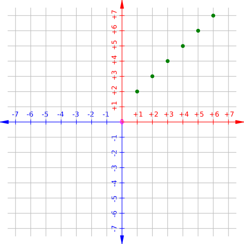
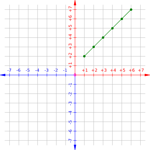
Now, what if we were to treat the x's and y's within this table as ordered pairs? We would get a bunch of points on the Cartesian plane:
...and if we were to connect all of these points together, then we would get a line:
This process is called "graphing" and it is one of the purposes of the Cartesian plane. It allows us to turn shapes into equations, and equations into shapes! [The fancy mathematical term for this activity is "analytic geometry". In this context, "analysis" generally means to represent something with numbers.] In particular, this type of equation is called a "linear function" because it makes a line when we graph it.
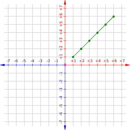
If we look carefully, we see that both columns within the above table are the counting numbers. To put it another way, the numbers in the y column are the exact same sequence of numbers as those in the x column just shifted up by 1 (our common difference). What would happen if we made x = y? It would make this graph:
Compare this with the previous graph. It is as if we slid the entire line downward by 1. However, the relationship between the points themselves has not been altered because x and y are still changing by the same amount! This movement is generally referred to as a "translation" of the graph.
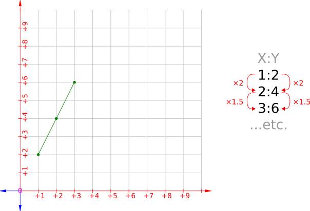
Let's try graphing another equation. For example:
2x = y
This represents the powers of two that we have encountered before. We will make another table for different values of x and y to make it easy to see:
| x |
y |
| 1 |
2 |
| 2 |
4 |
| 3 |
8 |
| 4 |
16 |
| 5 |
32 |
| 6 |
64 |
| 7 |
128 |
| etc. |
etc. |
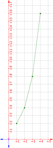
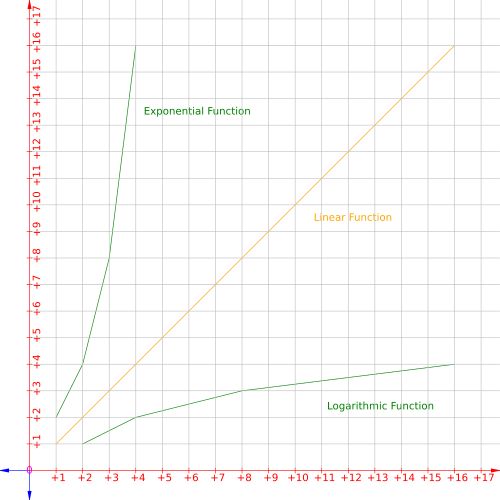
We will graph out these numbers as if they were a collection of ordered pairs. Because the numbers are so large, we will only do a few of them and focus in on only part of the Cartesian plane:
This type of equation (2x = y) is called an "exponential function" because it has an exponent (i.e.: the x). Unlike the linear function, it makes a curve when we graph it.
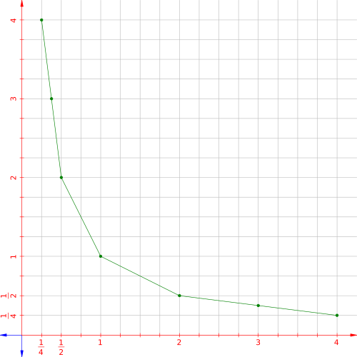
Let's try graphing out one last equation. For example:
log2 (x) = y
Again, we will make a table for different values of x and y to make it easy to see:
| x |
y |
| 2 |
1 |
| 4 |
2 |
| 8 |
3 |
| 16 |
4 |
| 32 |
5 |
| 64 |
6 |
| 128 |
7 |
| etc. |
etc. |
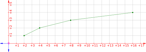
Did you notice something? All of the numbers are the same as those within the previous table, but the columns are switched! This is because exponentiation and logarithms are inverse operations. What happens when we graph the numbers in this table as if they were ordered pairs? Because the numbers are so large, we will only do a few of them and focus in on only part of the Cartesian plane:
This type of equation (log2 (x) = y) is called a "logarithmic function" because it is made from a logarithm. Like the exponential function, it makes a curve when we graph it. In this case, the graph for the exponential function and the graph for the logarithmic function are mirror images of one another. It is as if they were flipped across the linear function that we graphed before (i.e.: x = y)! To demonstrate:
This type of flipping is generally referred to as a "reflection" of a graph. Both translation and reflection are called "function transformations". They help us to change the graph of a function, or vice versa. There are other kinds of function transformations, but the important thing that we would like to emphasize here is how interconnected the functions and their graphs are. By changing one, we change the other.
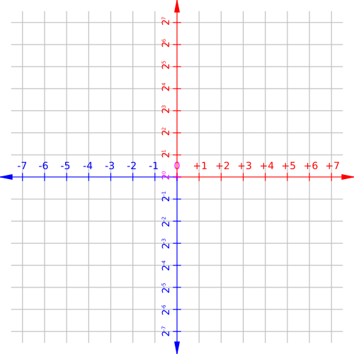
Now, what if we were to change the Cartesian plane itself? Before we try this, let's take a look at our number line again:
We know that moving to the right or left along the number line would be like adding or subtracting 1. Notice how similar this is to the arithmetic sequence that we described before. We would say that this number line follows a "linear scale". We can also make a number line where moving to the right and left would be equivalent to multiplying and dividing. For example:
The origin of this number line is 1 instead of 0, and moving to the right or left would be equivalent to multiplying or dividing by 2. Notice how similar this is to the geometric sequence that we described before. We would say that this number line follows a "logarithmic scale". We could also represent each point on this number line as a power of two, like so:
To the right are powers of two with positive exponents, and to the left are powers of two with negative exponents. The idea of a "negative exponent" may seem utterly bizarre. How does one multiply something by itself "negative times"? Instead of twisting our brain into knots trying to comprehend it, it is easier to think of it as simply asking us to divide that many times. For example:
23 = 1 × 2 × 2 × 2
and
2-3 = 1 ÷ 2 ÷ 2 ÷ 2
This is why the negative exponents are representing decimals in the above number line. For example:
2-1 = 0.5
2-2 = 0.25
2-3 = 0.125
2-4 = 0.0625
2-5 = 0.03125
...etc.
The same methods that we used for multiplying and dividing larger numbers by adding and subracting smaller ones will still work too! To give an example...
2-2 × 2-3 = 2(-2)+(-3) or 2-5
which is the same as
0.25 × 0.125 = 0.03125
We can see how connected arithmetic and geometric progressions are, much like addition and multiplication, or multiplication and exponentiation.
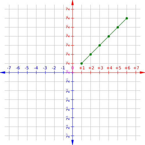
Now, let's take two number lines (one following a logarithmic scale and another following a linear scale) and make a Cartesian plane with them like before:
In this case, the Y-axis is the number line with a logarithmic scale, and the X-axis is the number line with a linear scale. If we graph out our exponential function on this plane, then we get this:
This is referred to as a "semi-log plot". Notice that it has turned the curve of the exponential function into a line!
It would seem that all of these things are deeply intertwined: the function, the graph it makes, and the coordinate system in which it is graphed. If we change one, then we simultaneously affect the other two, even if we may not always be aware of doing so.
...Let's get back to our arithmetic progression for a moment. Again, it is just the regular counting numbers:
1, 2, 3, 4, 5, 6, 7, 8, 9, etc.
Therefore, we could make other arithmetic progressions merely by "skip counting" by other numbers. To give a few examples:
We can count by 2's...
2, 4, 6, 8, 10, 12, 14, 16, 18, etc.
This is an arithmetic progression with a common difference of 2 (as we are just adding 2 repeatedly). We can also refer to them as "multiples" of 2.
Likewise, we could skip count by 3's or 4's...
3, 6, 9, 12, 15, 18, 21, 24, 27, etc.
4, 8, 12, 16, 20, 24, 28, 32, 36, etc.
These would be arithmetic progressions with common differences of 3 and 4, respectively. We could also refer to them as "multiples" of 3 and 4.
We can continue this pattern however high that we wish, but there is a simple way to refer to all of them simultaneously, through a "multiplication table":
| × |
1 |
2 |
3 |
4 |
5 |
6 |
7 |
8 |
9 |
| 1 |
1 |
2 |
3 |
4 |
5 |
6 |
7 |
8 |
9 |
| 2 |
2 |
4 |
6 |
8 |
10 |
12 |
14 |
16 |
18 |
| 3 |
3 |
6 |
9 |
12 |
15 |
18 |
21 |
24 |
27 |
| 4 |
4 |
8 |
12 |
16 |
20 |
24 |
28 |
32 |
36 |
| 5 |
5 |
10 |
15 |
20 |
25 |
30 |
35 |
40 |
45 |
| 6 |
6 |
12 |
18 |
24 |
30 |
36 |
42 |
48 |
54 |
| 7 |
7 |
14 |
21 |
28 |
35 |
42 |
49 |
56 |
63 |
| 8 |
8 |
16 |
24 |
32 |
40 |
48 |
56 |
64 |
72 |
| 9 |
9 |
18 |
27 |
36 |
45 |
54 |
63 |
72 |
81 |
This is a 9 × 9 multiplication table. We don't need one any larger than this because 9 is the largest single digit number in base-ten. Anytime that we have one more than 9 in a place value, then we add another digit to our numeral. For example:
9 + 1 = 10, which is a 2-digit number
99 + 1 = 100, which is a 3-digit number
999 + 1 = 1000, which is a 4-digit number
...etc.
Therefore, it is the same ten symbols cycling over and over again. To continue...
You are probably already thoroughly familar with how to use a multiplication table, but to give a quick example:
If we wanted to find 8 × 7, first we would find the row corresponding to 8, our "multiplier"...
| × |
1 |
2 |
3 |
4 |
5 |
6 |
7 |
8 |
9 |
| 1 |
1 |
2 |
3 |
4 |
5 |
6 |
7 |
8 |
9 |
| 2 |
2 |
4 |
6 |
8 |
10 |
12 |
14 |
16 |
18 |
| 3 |
3 |
6 |
9 |
12 |
15 |
18 |
21 |
24 |
27 |
| 4 |
4 |
8 |
12 |
16 |
20 |
24 |
28 |
32 |
36 |
| 5 |
5 |
10 |
15 |
20 |
25 |
30 |
35 |
40 |
45 |
| 6 |
6 |
12 |
18 |
24 |
30 |
36 |
42 |
48 |
54 |
| 7 |
7 |
14 |
21 |
28 |
35 |
42 |
49 |
56 |
63 |
| 8 |
8 |
16 |
24 |
32 |
40 |
48 |
56 |
64 |
72 |
| 9 |
9 |
18 |
27 |
36 |
45 |
54 |
63 |
72 |
81 |
Then, we would find the column corresponding to 7, our "multiplicand"...
| × |
1 |
2 |
3 |
4 |
5 |
6 |
7 |
8 |
9 |
| 1 |
1 |
2 |
3 |
4 |
5 |
6 |
7 |
8 |
9 |
| 2 |
2 |
4 |
6 |
8 |
10 |
12 |
14 |
16 |
18 |
| 3 |
3 |
6 |
9 |
12 |
15 |
18 |
21 |
24 |
27 |
| 4 |
4 |
8 |
12 |
16 |
20 |
24 |
28 |
32 |
36 |
| 5 |
5 |
10 |
15 |
20 |
25 |
30 |
35 |
40 |
45 |
| 6 |
6 |
12 |
18 |
24 |
30 |
36 |
42 |
48 |
54 |
| 7 |
7 |
14 |
21 |
28 |
35 |
42 |
49 |
56 |
63 |
| 8 |
8 |
16 |
24 |
32 |
40 |
48 |
56 |
64 |
72 |
| 9 |
9 |
18 |
27 |
36 |
45 |
54 |
63 |
72 |
81 |
Finally, we see where these rows and columns "intersect" (or cross) to get the result, our "product". In this case, our product is 56. So, 8 × 7 = 56.
However, instead of using this table to multiply, we are going to find the digital roots of all of our products, like this:
| * |
1 |
2 |
3 |
4 |
5 |
6 |
7 |
8 |
9 |
| 1 |
1 |
2 |
3 |
4 |
5 |
6 |
7 |
8 |
9 |
| 2 |
2 |
4 |
6 |
8 |
1 |
3 |
5 |
7 |
9 |
| 3 |
3 |
6 |
9 |
3 |
6 |
9 |
3 |
6 |
9 |
| 4 |
4 |
8 |
3 |
7 |
2 |
6 |
1 |
5 |
9 |
| 5 |
5 |
1 |
6 |
2 |
7 |
3 |
8 |
4 |
9 |
| 6 |
6 |
3 |
9 |
6 |
3 |
9 |
6 |
3 |
9 |
| 7 |
7 |
5 |
3 |
1 |
8 |
6 |
4 |
2 |
9 |
| 8 |
8 |
7 |
6 |
5 |
4 |
3 |
2 |
1 |
9 |
| 9 |
9 |
9 |
9 |
9 |
9 |
9 |
9 |
9 |
9 |
Remember, just repeatedly add the digits together until you get a single-digit number.
This is called a "Cayley table". It tells us many things about how a set of items (in this case, the digits 1 through 9) can interact with one another. We aren't going to cover it too deeply just yet, but we would like to point out one very important property:
Notice that some rows and columns within the table are mirrored from one another. For example, the sequence derived from multiples of 8 is actually the reverse of the sequence derived from multiples of 1. The same is true for 2-7, 3-6, and 4-5.
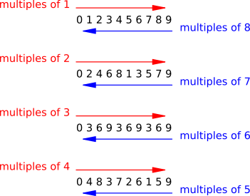
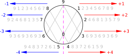
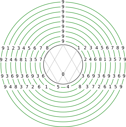
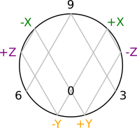
These are The Polar Number Pairs that we encountered before! Let's see them on The Fingerprint of God diagram:
Again, each of the sequences on the left are the reverse of those on the right. For example, the sequence derived from the multiples of 2 goes up by 2, while the sequence derived from the multiples of 7 goes down by 2. This is why each of the arrows are labeled with numbers that have a positive sign (+) or a negative sign (-).
Even though we have drawn The Fingerprint of God diagram on a flat surface, it is not actually 2-dimensional, it is technically 1-dimensional. In other words, it is as if we folded the number line in on itself to form a ring! [The fancy mathematical term for this process is "compactification". We have taken something that would normally be considered "infinite" and made it "finite".]
In order to see how this idea affects our 2-dimensional coordinate system, we have to introduce a few more concepts...
Part 2: The Basics of Tessellations
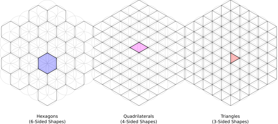
Like the tiles on the floor and/or walls of most bathrooms, only certain shapes can pack together, or "tessellate", to completely cover a surface without gaps. These are called "tessellations" or "tilings", and some of the most basic ones are the "Regular Tilings". They are made by repeating a single shape over and over again. For example:
The prefix "hex-" means "six", the prefix "quad-" means "four", and the prefix "tri-" means "three".
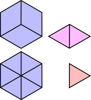
Notice that all of these shapes can be converted into one another:
• A hexagon is 3 quadrilaterals.
• A quadrilateral is 2 triangles.
• A hexagon is 6 triangles.
In general, any shape can be divided into triangles, so any one of these tilings could serve our purposes. But for now, we are looking for a specific type of 4-sided shape called a "Golden Rhombus"...It looks like it is time for us to do another construction!
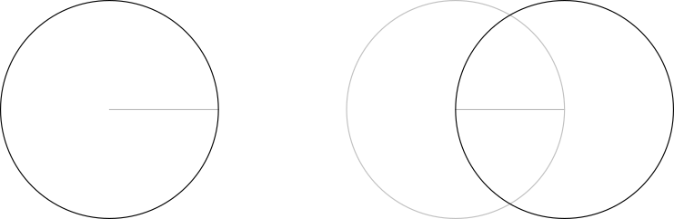
Step 1: Decide on a width for each tile and draw a line to represent this width.
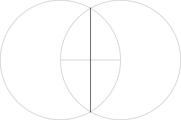
Step 2: Using this line as a radius, draw a circle on both ends of it.
Step 3: Using the points where the two circles overlap, draw another line perpendicular to the first.
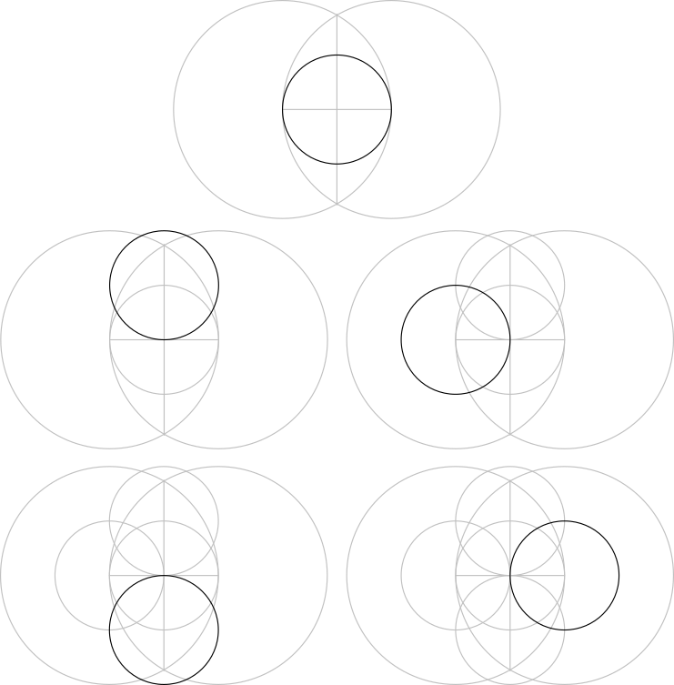
Step 4: Where the two lines intersect, draw a circle in the center and four circles around it of the same size.
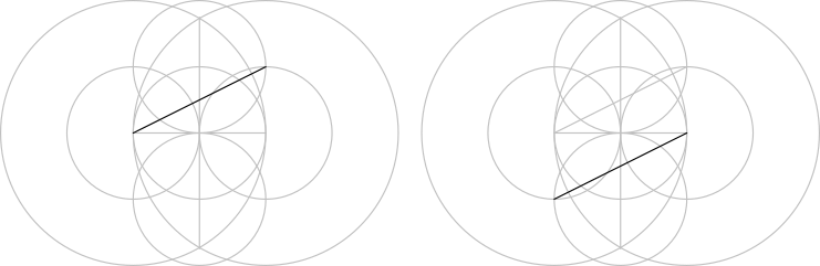
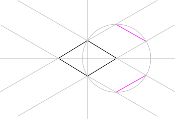
Step 5: Use the petal-like shapes where the circles overlap to draw two diagonal lines.
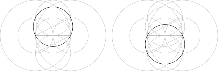
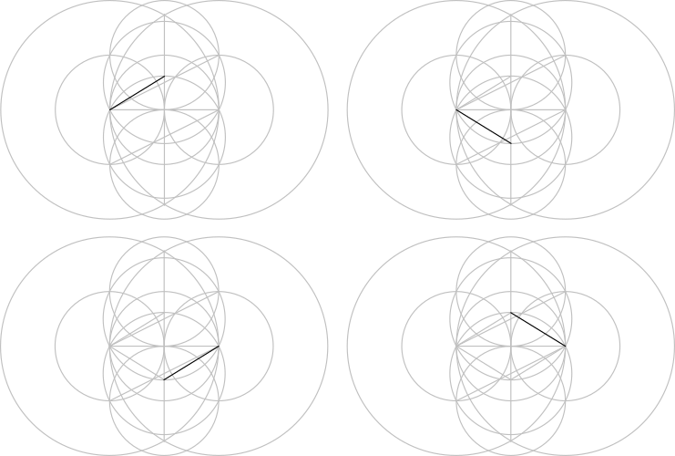
Step 6: Use where the diagonal lines cross the vertical line to draw two more overlapping circles.
Step 7: Connect the four points made by the two circles in previous step into the following pattern:
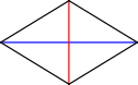
This is a single tile within our grid. It is called a "Golden Rhombus" because the diagonals are in a Golden Mean Proprotion φ (shown here by the red and blue lines).
Step 8: We can make any size grid that we need by extending the lines in all directions and continuously making circles in order to divide those lines into regular intervals.
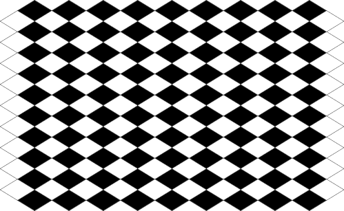
Step 9: We are going to make a 9 × 9 grid and remove all of the guidelines.
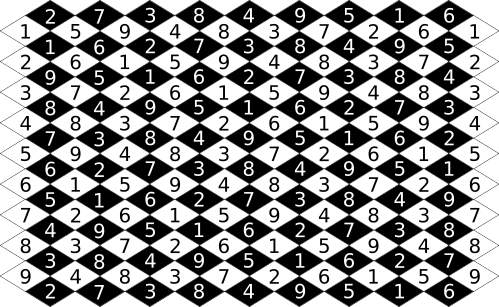
We will refer to this grid as The Diamond Grain. It will act like a "lattice" or framework to hold our numbers. Because we are using integers, there is a "polarity" (i.e.: a pattern of negative and positive) inherent to the grid itself. This polarity will be represented by coloring the diamond-shapes black and white, like a chessboard:
Next, we will assign numbers to each tile, almost like playing a game of Sudoku...
We are only using the numbers 1 through 9 within the grid for the same reason that we only needed a 9 × 9 multiplication table earlier: 9 is the largest single digit number within base-ten, and we cycle through those ten symbols over and over again to represent larger numbers. However, it is important to note that since we are using integers, there are technically 18 distinct numerals used here (i.e.: positive 1-9 and negative 1-9).
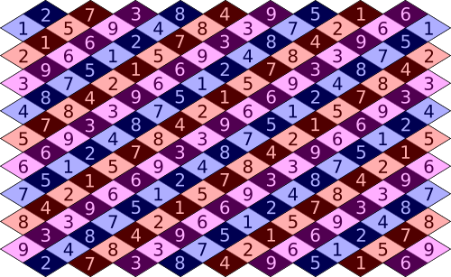
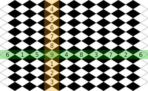
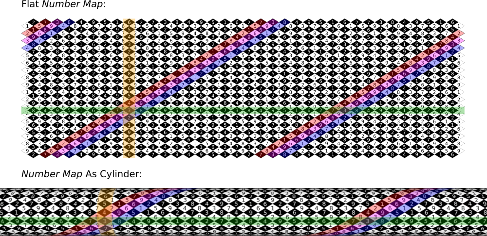
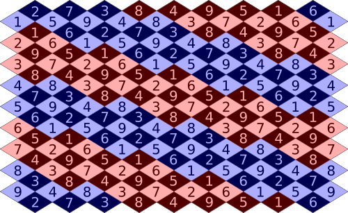
When we show the numbers within The Diamond Grain in this way, it will be called a Number Map. The relationships between the numbers in this Number Map are not arbitrary. It takes all of the patterns inherent to The Fingerprint of God diagram and expresses them along a flat surface instead of just a line!
For example, the two main number sequences associated with The Fingerprint of God are visible when moving diagonally from the bottom-left to the upper-right through the Number Map, or vice versa:
The Doubling-Halving Circuits (1-2-4-8-7-5 when seen forwards, and 5-7-8-4-2-1 when seen backwards) are marked here in red and blue, while The Gap Spaces (3-9-6-6-9-3) that lie between them are highlighted in magenta.
You have probably already noticed, but the geometric progression that we used earlier (i.e.: the powers of 2) is equivalent to The Doubling-Halving Circuit. Similar to how the graph of the exponential function changed from a curve into a line when we graphed it on a semi-log plot, The Doubling-Halving Circuit also makes a diagonal line on our Number Map!
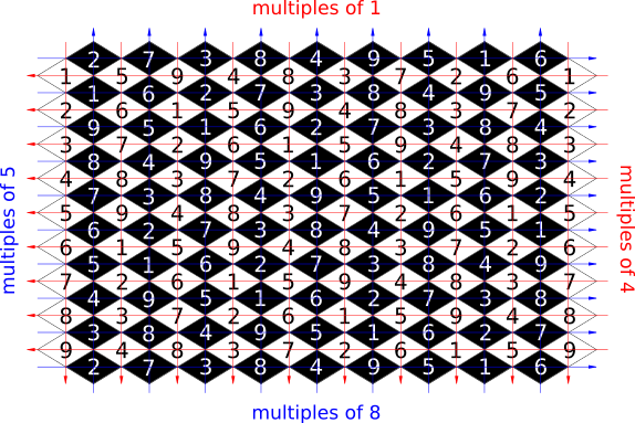
Further, every vertical line of tiles is the multiplication sequence associated with Polar Number Pair 1-8, while every horizontal line of tiles is the multiplication sequence associated with Polar Number Pair 4-5:
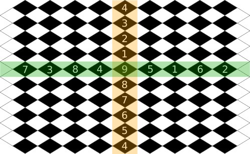
Remember, 9 and 0 are equivalent whenever we use a modulus of 9. Therefore, if 9 is considered an origin, then the 4-5 and 1-8 Polar Number Pairs would be like our X and Y axes. For example, here is just one set of axes highlighted within the Number Map:
The X-axis is shown here in green, while the Y-axis is shown in orange. We are only using negative tiles in the image above, but we could use positive tiles too. For example:
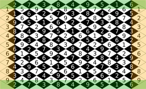
It is as if we took two Cartesian planes, one dedicated soley to positive numbers and another dedicated soley to negative numbers, and wove them together. This is called The Dual Non-Cartesian Coordinate System. Every tile within the Number Map is a point, and every line of tiles represents the graph of a function. The overall relationship of the numbers never changes, but the pattern that they make continuously repeats. While it may seem incredibly strange, we will try to demonstrate why it is important...
Notice that the top and bottom edges, as well as the left and right edges, are the exact same sequences of numbers:
This property allows us to represent every point in the plane with a single integer (instead of an ordered pair), and every graph will come back to meet itself in a loop! [Because all of the numbers within our functions eventually repeat, we would call them "periodic" (i.e.: they make "periods" or cycles), and because none of their graphs have breaks, we would call them "continuous" (i.e.: they "continue" rather than stop).] Let's use an analogy to help clarify...
Have you ever played the video game "Asteroids"? In this game, the player pilots a spaceship and shoots at asteroids. The entire game takes place on a single screen. If we fly off of the edge of it, then we immediately appear on the opposite edge of the screen as if they were connected:
Photo Credit: LibreTexts
[If we would like to give it a fancy name, then we could say that it has a "periodic boundary condition".] The Dual Non-Cartesian Coordinate System does the same thing. Any line of tiles going off the edge will come back to meet itself on the opposite edge!
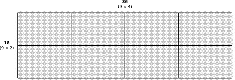
We are also not limited to a 9 × 9 Diamond Grain. Like the number line, all tilings are "infinite" in that they can be continuously extended in all directions in order to cover larger and larger surfaces. The Number Map can be tiled to any size that is needed just by adding another group of 9 in any direction in the same manner. There is a particular size that we will focus on here though, an 18 × 36 grid (made with eight copies of the 9 × 9 Number Map):
This will be referred to as One Quantum of 36. It is okay if not all of the numbers are visible within the above image. For now, we just want to give a general impression of what it looks like and point out one feature of it: The number of tiles within the vertical Y-axis is 9 × 2 = 18, while the number of tiles within the horizontal X-axis is 9 × 4 = 36. One is double the other. Hopefully, why this specific size is important will become apparent as we continue...
Part 3: The Basics of Topological Vector Spaces
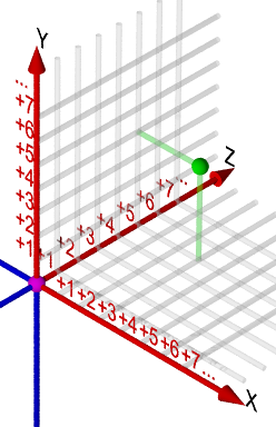
We can add another number line to our original 2-dimensional Cartesian plane. In addition to our X and Y axes, we now have a Z-axis that is perpendicular to them both, like this:
This is called a "3-dimensional Cartesian coordinate system", because it takes three coordinates or dimensions (x, y, z) to specify the location of any point within it. Similar to an ordered pair, we use a set of three numbers enclosed within parentheses and separated by commas to describe that point. For example, the coordinate (3, 4, 5) would represent this point:
The green dot is at coordinate (3, 4, 5). We've gone 3 units to the right along the X-axis, 4 units up along the Y-axis, and 5 units forward along the Z-axis away from the origin.
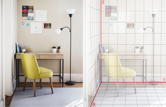
We can use this 3-dimensional system much like how we used our 1-dimensional number line or our 2-dimensional Cartesian plane. We can still use it to graph out relationships, turn shapes into equations or equations into shapes, and to model different kinds of situations. For example, let's use it to represent a room, with the back-left corner as our origin:
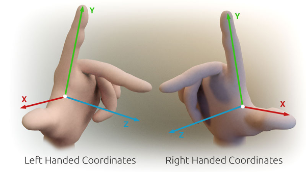
It is very important to understand the orientation of the axes relative to one another first. In other words, always look carefully at how the axes are labeled. Which axis is which? There are only two types of orientations, "left-handed" and "right-handed":
Photo Credit: Primalshell
In the case of the room, the X and Y axes describe the length and width of it, while the Z-axis describes its height. Therefore, we can pinpoint the location of anything within the room with three coordinates, even if it were an object that was floating up in the air. These three numbers would represent the distance of the object from each wall and its height above the floor starting from the origin.
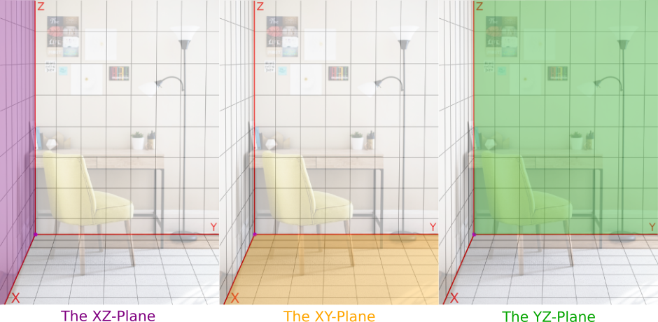
It is as if we put three 2-dimensional Cartesian planes together, with all of their origins meeting in the back-left corner of the room. Here is each one of these planes highlighted for sake of clarity:
Notice that if we only wanted to describe the location of something on the surface of one of these planes, then we would only need two coordinates. To give a couple of examples:
• It only takes an X and a Y coordinate to describe something on the XY-plane, such as where a leg of the chair contacts the floor.
• It only takes a Y and a Z coordinate to describe something on the YZ-plane, such as where a poster is on the back wall.
...etc.
Not enough lines? We can also scale the size of our grids to any amount of accuracy that we need by using more numbers within our number lines! For example:
Here we are doubling the amount of numbers used in our X and Y axes to give a finer resolution to the grid within the XY-plane.
In short, we have a system that will allow us to describe the locations of things within a given space with as much detail as is necessary.
We will come back to the concept of 3-dimensions, but for now, let's consider motion...
Motion can be thought of as represented by an arrow. The length of the arrow would symbolize the distance that an object travels in a given moment, and the direction that the arrow points would be the direction in which that object travels. This is called a "vector". For example:
The green arrow represents a "1-dimensional vector". It is "1-dimensional" because it exists on a number line. This particular 1-dimensional vector is describing the motion of a car to the right. A longer arrow would represent a faster motion to the right. In other words, the car would be covering more distance in less time.
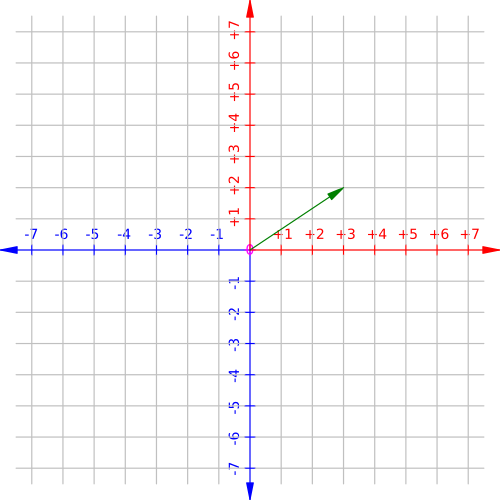
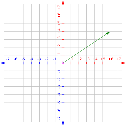
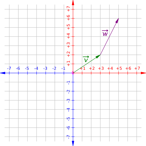
The "tail" of the arrow is called the "initial point", while the "head" of the arrow is called the "terminal point". If we think of the initial point as sitting on the origin of a Cartesian plane, then we can represent the vector as a pair of numbers stacked vertically within a square bracket. This is called a "matrix". It is similar to how a point is represented by an ordered pair. In this case, the top number describes how far the terminal point of the vector is horizontally from the origin (like the x-coordinate), and the bottom number describes how far the terminal point of the vector is vertically from the origin (like the y-coordinate). For example:
The green arrow is the vector  . Notice that, when they are taken together, the two numbers tell us both the length and direction of the vector. Therefore, this is a "2-dimensional vector". Let's play with it...
What if we were going twice as fast within a given moment? Then our vector would be twice as long. For example:
The green arrow has now become the vector  . It is twice as long as it was previously.
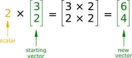
How did we get this new vector? We multiplied all of the numbers within the matrix by 2, like this:
Whatever number that we multiply a matrix by is called a "scalar". It is called a "scalar" because it scales whatever the matrix is describing up or down in size. In this case, 2 is our scalar, and it doubled the length of our vector. This process is called "scalar multiplication". To reiterate:
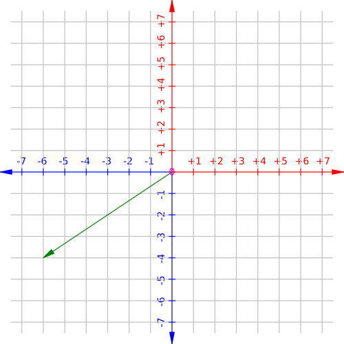
If the scalar was a negative number, then it would flip the direction of the vector. For example:
...and on the Cartesian plane, we would end up with this:
If we had a set of movements one after another, then we could represent each of them as a vector and add them together to show where we would end up. This process is called "vector addition".
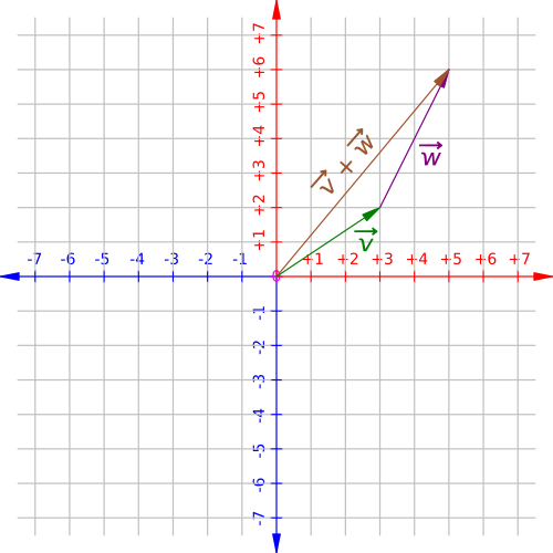
For example, let's take the vectors and  . We will put the matrix for each vector in a row and add up the numbers within them horizontally:
On the Cartesian plane, this is equivalent to placing all of the vectors end-to-end, like this:
Here, each vector is given a letter name to distinguish them from one another, and each of the letters also has a little arrow above it to specify that it is the name of a vector. Even though the initial point of vector  is no longer on the origin, it still moves 2 over and 4 up, just as its matrix indicates!
In general, vector addition gives us a new vector that symbolizes where we would end up after all of those movements have been completed. To continue the above example...
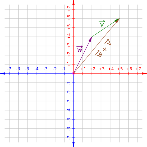
Also, notice that it doesn't matter which vector comes first. We could have started with instead of and we still would have come to the same result:
Therefore, vector addition is commutative.
The main thing that we would like to point out is that one can do operations on vectors much like "regular" numbers. [The matrices of vectors can also be used in ways that are similar to the ideas of "functions" and the "transformations" that we did on their graphs in Part 1. These are called "linear transformations".]
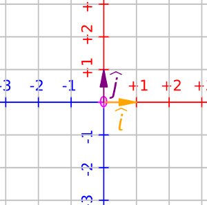
Let's make two vectors, one on each axis, and both with a length of 1 unit:
Each of these vectors has a name, the letters i and j with a little carrot (^) over them. They are read as "i-hat" and "j-hat", respectively. These are called "basis vectors". By scaling and adding them, we can reach any point within the plane. Whenever we scale and add a pair of vectors like this, it is referred to as a "linear combination". All of the points that we can reach with it are referred to as the "span" of those vectors.
Every point within the plane can also be thought of as a vector and/or combination of vectors. When we are referring to all of them together, this is called a "vector space". In short, the 18 × 36 Number Map can be thought of as a vector space, and we can use it to describe the motion of objects directly!
In order to do this, imagine that it was a sheet of rubber that we could bend without tearing. [This type of thinking is common a branch of mathematics called "topology", which explores how we can change the form of something without changing its function.] We can roll the 18 × 36 Number Map into a tube-like shape (a "cylinder"), and then roll that tube into a doughnut-like shape (a "ring torus"). This process would look something like this:
Photo Credit: Kieff
[If we want a fancy way to describe this, then we could say that the set of numbers that make up each edge are "equivalence classes" that we mapped to each other to form a "quotient space". In other words, the numbers are the same in each, so we grouped them together.] Let's take this a step at a time, starting with the cylinder:
Each of The Doubling-Halving Circuits (shown in red and blue), and each of The Gap Spaces (shown in magenta), have become a spiral-like shape (a "helix"). Likewise, all of our Y-axes (shown in orange) have changed from lines into circles! [Notice how similar this is to the "compactification" process that we did with our number line in Part 1! Again, we are taking something that would normally be considered "infinite" and making it "finite".]
We can see a representation of these rings within the multiplication sequences:
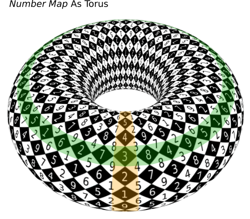
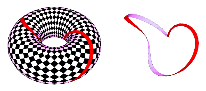
Next, there is the ring torus:
[The above diagram was made with the help of Chuck Middaugh's Parametric ABHA Torus Blender model.]
We will refer to this as The ABHA Torus. Like all of our Y-axes, all of our X-axes (shown in green) have also become rings!
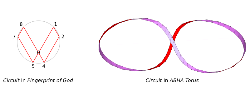
Something interesting happens with our Doubling-Halving Circuits and Gap Spaces. Let's ignore the numbers for a moment, and extract one of them to see its shape:
It may not seem like much, but a side-view shows its significance:
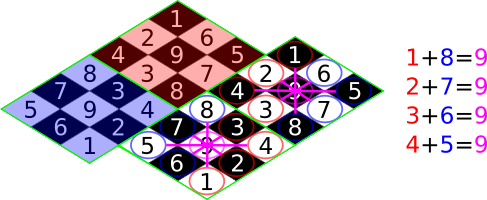
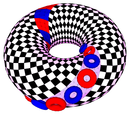
The Fingerprint of God and The ABHA Torus are two representations of the same system. For example, the zero is the hole of the torus! Likewise, since 0 and 9 are equivalent in a modulus of 9, every 9 on the Number Map is actually the hole of a smaller torus. The smaller tori are represented by little 3 × 3 squares called Nested Vortices:
Each of them contain the digits 1-9 and The Polar Number Pairs always mirror across the 9:
This means that The ABHA Torus is self-similar. It is a ring made of rings! Here are a set of Nested Vortices occuring over a pair of Doubling-Halving Cirucits and a Gap Space. One half of them are shown as a grid, and the other half are shown as actual rings:
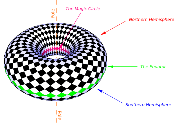
Each part of The ABHA Torus also has its own name:
• The central hole is The Magic Circle. The "pole" of the torus (shown with orange dashes) passes through it.
• The outer ring is The Equator. It divides the torus into two halves or "hemipsheres", the Northern Hemisphere and Southern Hemipshere.
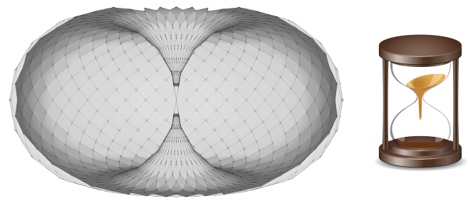
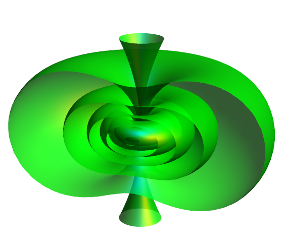
Let's play with it some more! We will squeeze The Magic Circle until it becomes a tiny hole. From the pole-view, it would look like this:
This makes it into a "horn torus". Here is a cross-section of one:
The trumpet-like shapes (or "hyperbolic cones") are the "horns". When referencing both of them at the same time, we will call them The Hourglass for their similarity in shape.
No matter how compressed The Magic Circle becomes, there will always be a hole there! This may seem like a trivial detail, but it is very important because The Magic Circle is the origin of a 3-dimensional coordinate system. In order to use it, we must first nest nine of The ABHA Tori inside one another. It will look something like this:
Photo Credit: Nested Tori
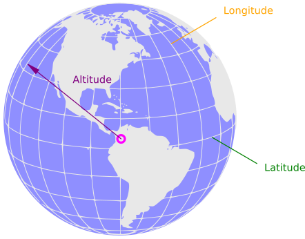
This property gives us a Z-axis that moves in-and-out "radially" (i.e.: in all directions simultaneously). While it may seem complicated, the principles behind it are simple. It works much like a globe:
• The "latitude" lines (moving from side-to-side along the surface) are equivalent to the X-axis represented by multiples of 4-5.
• The "longitude" lines (moving up-and-down along the surface) are equivalent to the Y-axis represented by multiples of 1-8.
• The "altitude" (moving in-and-out) is equivalent to the Z-axis represented by multiples of 2-7. This is like jumping from one torus to the next.
We have uncovered one way of using The Dual Non-Cartesian Coordinate System in 3-dimensions! Notice that we are also using all three of The Polar Number Pairs within The Doubling-Halving Circuit. We can represent this on The Fingerprint of God in the following manner:
[If we want to give it a fancy name, then we could refer to The ABHA Torus as a "manifold". In other words, while it may seem like a torus in 3-dimensions, all along its surface it acts like The Number Map in 2-dimensions. This is similar to the relationship between The Number Map and The Fingerprint of God. No matter how many dimensions we use, all of the patterns will always be retained!]
What makes this type of coordinate system special is that a single number automatically gives us all of the other numbers in every direction, and further, they make a geometry that is applicable to every level of scale...
Part 4: The Unified Field
According to the Encyclopedia Britannica, "physics" is:
The science that deals with the structure of matter and the interactions between the fundamental constituents of the observable universe. In the broadest sense, physics (from the Greek physikos) is concerned with all aspects of nature on both the macroscopic and submicroscopic levels.
Many scientists throughout history have added to our understanding of the world around us. Questions involving the movement of objects have been prevalent within this search for understanding. In order to answer these questions, we need to develop a language to describe how things move. Generally, motion is when an object changes locations within a given amount of time. It is measured as a "rate" (such as "miles per hour"). If we add a direction in which this rate is applied, we call it "velocity". Velocity can be represented as a vector because it is a speed with direction.
In the case of "free fall" (i.e.: when an object is falling and nothing else is acting on it, such as the "drag" of the air), it was found that velocity itself increases. This is called "acceleration". The "something" that causes this acceleration was named "gravity" (short for "gravitation"). We will get into the exact mechanisms behind the cause of gravity later, but for now, we will simply think of it as that which makes objects fall towards one another. Those objects are said to be "attracted" to each other.
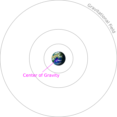
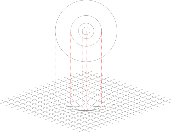
All objects are seen as having gravity. The strength of it changes depending upon the "density" of the object (i.e.: how much material there is packed into a given volume) and how far away we are from it. If we take the Earth as an example, a simple way to picture how the strength of gravity changes around it is by imagining it within a set of "concentric", or nested, spheres:
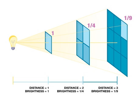
The center point, where gravitation seems strongest, is called a "center of gravity". All of the spheres around the object would be referred to as its "gravitational field". Notice that the strength of gravity becomes weaker the farther out we move. It follows a relationship called an "inverse square law". A simple way to think of it is this: If we double our distance from the center, the intensity of gravity is one-fourth as strong at that point because its influence is spread out over a larger area. This larger area is represented by a larger sphere.
This pattern actually applies to many things, such as the brightness of a light:
Photo Credit: Paul C. Buff
The light is getting dimmer as we move farther away from it.
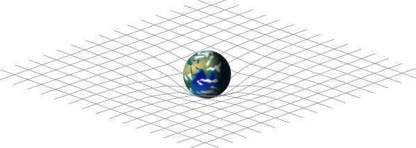
Other geometries can be used to describe gravity too! For example, we can use a flat sheet with a dimple in it:
Photo Credit: Mysid
This dimple is called a "gravity well". The deeper we move into the curve of the gravity well, the stronger the gravity is at that point. Notice that this model is essentially the same as using the concentric spheres:
Any object that falls into a gravity well has to be moving at a particular speed and in a particular direction in order to leave it. This is called an "escape velocity". The path that an object takes is a "trajectory". If that path repeatedly curves around another object, then it is in "orbit". A good example is the Moon revolving around the Earth:
Photo Credit: BestAnimations
A "force" is something that causes an acceleration. There are a pair of forces acting on an object to keep it rotating like this:
1. There is a "centripetal force" which pushes that object towards the center of its orbit (like gravity). This keeps it from flying off.
2. There is a "centrifugal force" which keeps that object continuing in its forward motion. Things have a tendency to continue in their trajectories unless something interacts with them. This is called "inertia".
A simplified way of thinking of these two forces is that, one is an attraction or push towards a center, while the other is a repulsion or push away from a center. The dynamic balance of these two forces is what keeps objects orbiting one another without crashing into each other.
An entire branch of mathematics was developed for understanding how things change over time (such as the position of an object within its trajectory). It is referred to as "calculus", and it is used extensively throughout science (especially physics) because everything in reality seems to be moving in some way. It involves the use of "differential equations" which can be used to describe a changing rate (like an acceleration)! We won't cover it too deeply here, but we would like to point out one of its applications: "differential geometry".
Differential geometry is a way of making shapes by moving curves through space. For example, we can create a torus by spinning a circle along the circumference of another circle that is 90-degrees away from it:
Photo Credit: Lucas Vieira
Therefore, a torus is sometimes called a "solid of revolution". We would like to use this same process to make another shape, but we have to find the curve that generates it first. In order to do that, we must take a brief detour into music again...
If we pluck the string of an instrument (such as a guitar), then we get a sound of a particular frequency. If we divide that string in half, then we get a sound with a frequency twice as fast. We can continue to do this (e.g.: dividing into three would make a sound with a frequency three times as fast, dividing it into four would make a sound with a frequency four times as fast, and so on). Notice the similarity of this process to the overtone series that we encountered before. Graphing it out would make this curve:
This is called a "rectangular hyperbola". Notice that the rectangular hyperbola is getting closer to the vertical and horizontal axes the farther out the curve is extended in both directions. [If we want to be extra-fancy, then we could say that the hyperbola is approaching the axes "asymptotically" as it goes to "infinity".]
Another simple way to think about this relationship is as a ratio between the number that represents the X-axis and the number that represents the Y-axis.
If both numbers increase or decrease at the same time, then it is called a "direct ratio". This relationship graphs as a line.
If one number increases while the other decreases, or vice versa, then it is a called an "inverse ratio". This relationship graphs as a rectangular hyperbola.
Can you see how this relates to The Doubling-Halving Circuit?
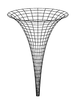
Rotating the rectangular hyperbola along the vertical axis produces a hyperbolic cone:
Photo Credit: Franz Fitzke
[This method of forming a hyperbolic cone was discovered by Walter Schauberger, son of the great naturalist, Viktor Schauberger. Walter attempted to put into mathematical form the patterns that his father had encountered throughout a lifetime of study into Nature. The hyperbolic cone is a shape that is very prevalent throughout Nature, particularly within the vortex motions of air and water. The fact that it is arising from this musical pattern is important!]
The flat sheet that we dealt with earlier is often referred to as "spacetime". It is called this because it combines space and time into a single concept. To give a very basic example, if we wanted to describe the motion of objects within this space, then we can add another coordinate to represent time (such as the the letter s to represent seconds). This would make our coordinate system "4-dimensional" because we are using four coordinates. This might sound as if it is something fantastic, but it is actually quite simple: Three coordinates (x, y, z) are used for describing where an object is, and one coordinate (s) is used for describing when it is there. There are other ways of interpreting spacetime and the concept of 4-dimensions, but this explanation will suffice for now.
Let's imagine that, instead of the gravity well being just a dimple, it was actually a hyperbolic cone. The "tip" of the hyperbolic cone is going towards "infinity", so the strength of gravity is thought to be "infinite" at that point. This is a "singularity", and when spacetime does this, it is called a "black hole".
Photo Credit: NUS Faculty of Science - Black holes with unusual horizons
Black holes are often thought of as something mysterious, but we won't dive into the details here. We only want to highlight the characteristic described above. We can even invert this pattern to make a "white hole". Generally, instead of an intense "pull" towards a center, it is the opposite, an intense "push" away from a center. We will still represent it by the same shape (i.e.: a hyperbolic cone).
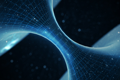
Let's take two hyperbolic cones, one representing a black hole and another representing a white hole. When they meet tip-to-tip, we get a structure called a "wormhole":
Photo Credit: Traveling Through a Wormhole May Be Possible - But It Wouldn't Be A Shortcut (Newsweek)
Notice the similarity of this shape to The Hourglass mentioned before. The horn torus allows us to take something that is considered "infinite" (e.g.: the curvature of the black hole) and make it "finite" by bending it until it comes back to meet itself in a loop! As it does so, it inverts to become a white hole, and together they form a wormhole. All of these are represented within The ABHA Torus.
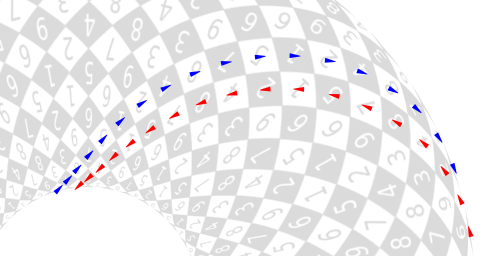
In fact, all of the patterns that we have covered thus far are present within The ABHA Torus in some way. For example, The Magic Circle can be thought of as a center of gravity, and the concentric spheres of the gravitational field are equivalent to the nested tori. If we pay attention only to the numbers for a moment, then we can see something interesting about The Doubling-Halving Circuits too:
The doubling going towards the center (marked by red arrows) is like acceleration due to gravity. The halving going outward (marked by blue arrows) is like the inverse square law. [Technically speaking, if we thought of each of these tiles as a vector, then they would be considered "linearly dependent" because they lead us back to the origin when they are added together.] Notice that these pathways are also curved, so they can be used to describe the centripetal and centrifugal forces as well.
It may seem strange to talk about the "shape of space", but the Universe itself (i.e.: the largest distance that we are able to measure) has a certain kind of geometry to its spacetime.
The Universe...
• is "multiply connected" (i.e.: a torus with a hole). This includes a horn torus with a tightly compressed hole.
• is "compact, without a boundary" (meaning that it is "finite" in extent, but has no edge). If we go out far enough, we end up back at the center, just like with the multiples of 2-7 for our Z-axis!
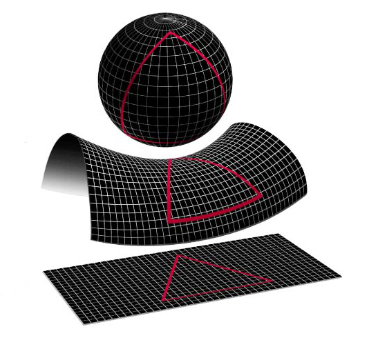
• has "positive", "negative", and "flat curvature"...
In this context, the term "curvature" has to do with how the spacetime is bending:
• "Positive Curvature" is like the surface of a sphere. The angles of a triangle on such a surface add up to more than 180-degrees.
• "Negative Curvature" is like a saddle shape. The angles of a triangle on such a surface add up to less than 180-degrees.
• "Flat Curvature" is like a flat plane. The angles of a triangle on such a surface add up to 180-degrees.
The ABHA Torus embodies all three of these curvatures. Its outer surface has positive curvature, the inner part (i.e.: The Hourglass) has negative curvature, and yet every part of it acts like a flat plane (i.e.: The Number Map)!
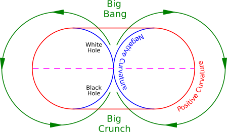
There are models which attempt to describe the evolution of the Universe (i.e.: how it unfolds from beginning to end). It is thought to have expanded from a highly dense and hot point. This is called "The Big Bang". Likewise, one of the theories as to what will eventually happen to it is the exact reverse (i.e.: all objects will collapse into a highly dense and hot point once more). This is called "The Big Crunch".
If we were to combine these ideas with The ABHA Torus, we can use it to describe the cyclic regeneration of the Universe as a whole (a kind of "steady-state")...
There are quite a few models that touch upon aspects of this mathematics and science in ways that are very similar. We will mention a couple of them here...
• Cristián Bredée's "Orange Theory":
There is a short video which gives a summary of this theory here. The "spiral trajectories" mentioned at 57 seconds into the video are equivalent to The Doubling-Halving Circuits.
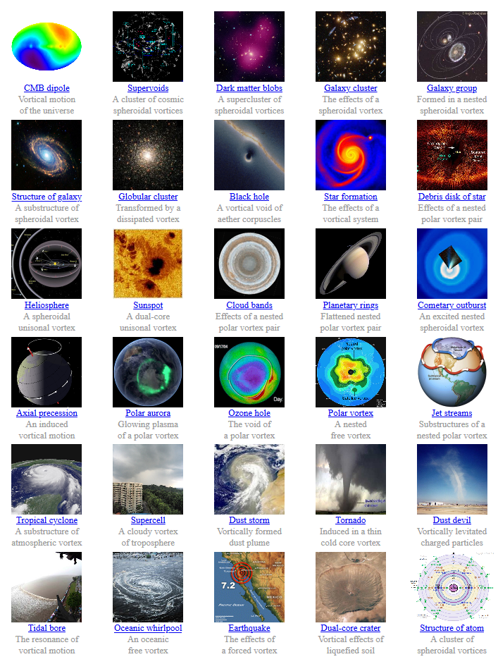
• Vincent Wee-Foo's "UVS Model":
Everything is made up of vortices and exists within vortices in some form. The Fingerprint of God is literally everywhere! There is nothing that the Creator does not touch.
The next article will give some ideas on how to apply this understanding to our technology.
Thank you for reading!